Asymsam

The Asymmetric and Symmetric SAM indices.

What is the Asymmetric SAM

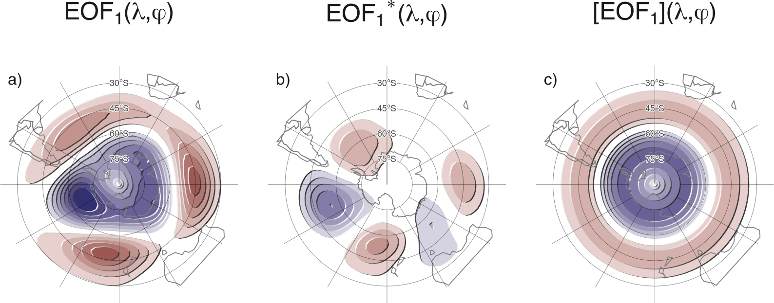
The Southern Annular Mode (SAM) is the main mode of variability in the Southern Hemisphere extratropical circulation (Rogers and van Loon 1982) on daily, monthly, and decadal timescales (Baldwin 2001; Fogt and Bromwich 2006) and exerts an important influence on temperature and precipitation anomalies, and sea ice concentration (e.g. Fogt and Marshall 2020). Its positive phase is usually described as anomalously low pressures over Antarctica surrounded by a ring of anomalous high pressures in middle-to-high latitudes, but on top of that zonally symmetrical description, the SAM holds noticeable deviations from zonal symmetry (Figure 1)

Three polar maps of the southern hemisphere. The first map is titled 'EOF1' and shows a pattern of low values near the center (high latitudes) and high values more to the sides (lower latitudes). The patterns are not completely ring-like. The area of high values have thre distinct local maxima arranged in equal distance. The area of low values has a single local minimum located to the left and between two of the local maxima mentioned before. The next map shows only three areas of high values and one area of low value which coincide with the local maxima and minima from the first figure. The third map shows a perfectly circular area of low values in the center and a perfect ring of high values surrounding it. — Figure 1: Regression of geopotential height (meters) at (row 1) 50~hPa and (row 2) 700~hPa with (column a) SAM, (column b) A-SAM, and (column c) S-SAM for the 1979 – 2018 period. The regression patterns for A-SAM and S-SAM are the result of one multiple regression using both indices. Points marked on panel b.2 are the location of the reference points used by Raphael (2004) for their Zonal Wave 3 index.

We derived a Asymmetric SAM index (A-SAM) and a Symmetric SAM (S-SAM) by computing the SAM as the leading EOF of geopotential height South of 20ºS (Fig. 1 a), splitting that field into it’s zonally asymmetric part (Fig. 1 b) and zonally symmetric part (Fig. 1 c) and finally projecting monthly geopotential fields onto each of these two new fields. The three indices are then normalized by dividing them by the standard deviation of the SAM index at each level. As a result, the magnitudes between indices are comparable, but only SAM index has unit standard deviation per definition.

Six maps similar to the ones before. They are arranged on a grid of two rows labeled "50 hPa" and "700 hPa" and three columns named "SAM", "A-SAM" and "S-SAM". The 700 hPa row shows three plots that are very similar to the ones in Figure 1. The main difference is that the last map (S-SAM) is not a perfect ring, and has some small deviations from a perfect circle. In the 50 hPa row, the first plot (SAM) shows a single and very intense area of low values at high latitudes which is slightly off-centre. ç The second plot (A-SAM) shows a dipole with low values to the right and high values to the left with the South Pole in between them. The third plot (S-SAM) is similar to the first but the shape is much closer to a circle and more closel-centered in the South Pole. — Figure 2: Regression of geopotential height (meters) at (row 1) 50~hPa and (row 2) 700~hPa with (column a) SAM, (column b) A-SAM, and (column c) S-SAM for the 1979 – 2018 period. The regression patterns for A-SAM and S-SAM are the result of one multiple regression using both indices. Points marked on panel b.2 are the location of the reference points used by Raphael (2004) for their Zonal Wave 3 index.

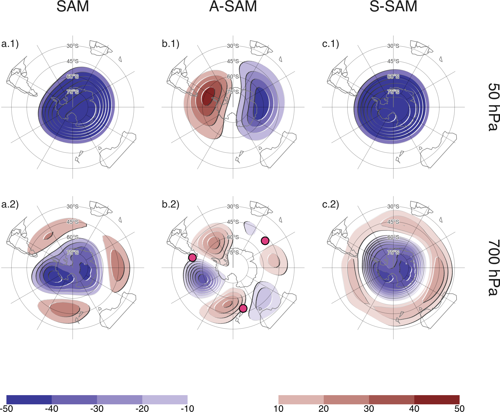
The resulting indices separate the zonally symmetric and zonally asymmetric part of the SAM (Figure 2) and are associated with different impacts on temperature and precipitation.

For more details, see Campitelli, Díaz, and Vera (2022) and the companion blog post.

Get the data

You can grab the monthly indices for the 1979 – 2018 period as used in Campitelli, Díaz, and Vera (2022) in csvy format here.

Real-time indices can be accessed via this form.

How to cite

If you use this data on your research, please cite it with

Campitelli, Elio, Leandro B. Díaz, and Carolina Vera. 2022. “Assessment of Zonally Symmetric and Asymmetric Components of the Southern Annular Mode Using a Novel Approach.” Climate Dynamics 58 (1): 161–78. https://doi.org/10.1007/s00382-021-05896-5.

Bibtex entry:

@article{campitelli2022,
  title = {Assessment of Zonally Symmetric and Asymmetric Components of the {{Southern Annular Mode}} Using a Novel Approach},
  author = {Campitelli, Elio and D{\'i}az, Leandro B. and Vera, Carolina},
  year = {2022},
  month = jan,
  journal = {Climate Dynamics},
  volume = {58},
  number = {1},
  pages = {161--178},
  issn = {1432-0894},
  doi = {10.1007/s00382-021-05896-5},
  langid = {english}
}

References

Baldwin, Mark P. 2001. “Annular Modes in Global Daily Surface Pressure.” Geophysical Research Letters 28 (21): 4115–18. https://doi.org/10.1029/2001GL013564.

Campitelli, Elio, Leandro B. Díaz, and Carolina Vera. 2022. “Assessment of Zonally Symmetric and Asymmetric Components of the Southern Annular Mode Using a Novel Approach.” Climate Dynamics 58 (1): 161–78. https://doi.org/10.1007/s00382-021-05896-5.

Fogt, Ryan L., and David H. Bromwich. 2006. “Decadal Variability of the ENSO Teleconnection to the High-Latitude South Pacific Governed by Coupling with the Southern Annular Mode.” J. Climate 19 (6): 979–97. https://doi.org/10.1175/JCLI3671.1.

Fogt, Ryan L., and Gareth J. Marshall. 2020. “The Southern Annular Mode: Variability, Trends, and Climate Impacts Across the Southern Hemisphere.” WIREs Climate Change 11 (4): e652. https://doi.org/10.1002/wcc.652.

Raphael, M. N. 2004. “A Zonal Wave 3 Index for the Southern Hemisphere.” Geophysical Research Letters 31 (23). https://doi.org/10.1029/2004GL020365.

Rogers, Jeffery C., and Harry van Loon. 1982. “Spatial Variability of Sea Level Pressure and 500 Mb Height Anomalies over the Southern Hemisphere.” Mon. Wea. Rev. 110 (10): 1375–92. https://doi.org/10.1175/1520-0493(1982)110<1375:SVOSLP>2.0.CO;2.